Image Classification
=======================
The source code for this chapter is in [book/image_classification](https://github.com/PaddlePaddle/book/tree/develop/03.image_classification). For users new to book, check [Running This Book](https://github.com/PaddlePaddle/book/blob/develop/README.md#running-the-book) .
## Background
Compared with words, images provide information in a much more vivid, artistic, easy-to-understand manner. They are an important source for people to express and exchange ideas. In this chapter, we focus on one of the essential problems in image recognition -- image classification.
Image classification is the task of distinguishing images in different categories based on their semantic meaning. It is a core problem in computer vision and is also the foundation of other higher level computer vision tasks such as object detection, image segmentation, object tracking, action recognition. Image classification has applications in many areas such as face recognition, intelligent video analysis in security systems, traffic scene recognition in transportation systems, content-based image retrieval and automatic photo indexing in Internet services, image classification in medicine industry.
To classify an image we firstly encode the entire image using manual or learned features and then determine the category using a classifier. Thus, feature extraction plays an important role in image classification. Prior to deep learning the BoW(Bag of Words) model was the most widely used method for classifying an image. The BoW technique was introduced in Natural Language Processing where a training sentence is represented as a bag of words. In the context of image classification, the BoW model requires constructing a dictionary. The simplest BoW framework can be designed in three steps: **feature extraction**, **feature encoding** and **classifier design**.
With Deep learning, image classification can be framed as a supervised or unsupervised learning problem that uses hierarchical features automatically without any need for manually crafted features from the image. In recent years, Convolution Neural Networks (CNNs) have made significant progress in image classification. CNNs use raw image pixels as input, extract low-level and high-level abstract features through convolution operations, and directly output the classification results from the model. This style of end-to-end learning has led to not only higher performance but also wider adoption in various applications.
In this chapter, we introduce deep-learning-based image classification methods and explain how to train a CNN model using PaddlePaddle.
## Requirement
1. PaddlePaddle version 1.6 or higher, or suitable develop version.
## Result Demo
Image Classification can be divided into general image classification and fine-grained image classification.
Figure 1 shows the results of general image classification -- the trained model can correctly recognize the main objects in the images.
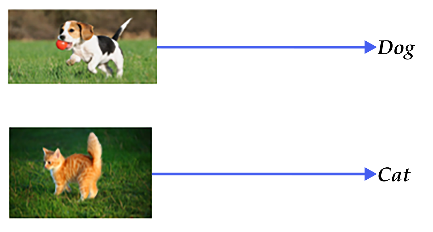
Figure 1. General image classification
Figure 2 shows the results of a fine-grained image classifier. This task of flower recognition ought to correctly recognize of the flower's breed.
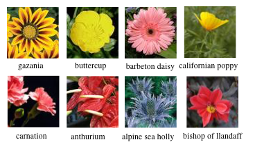
Figure 2. Fine-grained image classification
A qualified model should recognize objects of different categories correctly. The results of such a model should remain accurate in different perspectives, illumination conditions, object distortion or occlusion (we refer to these conditions as Image Disturbance).
Figure 3 shows some images with various disturbances. A good model should classify these images correctly like humans.
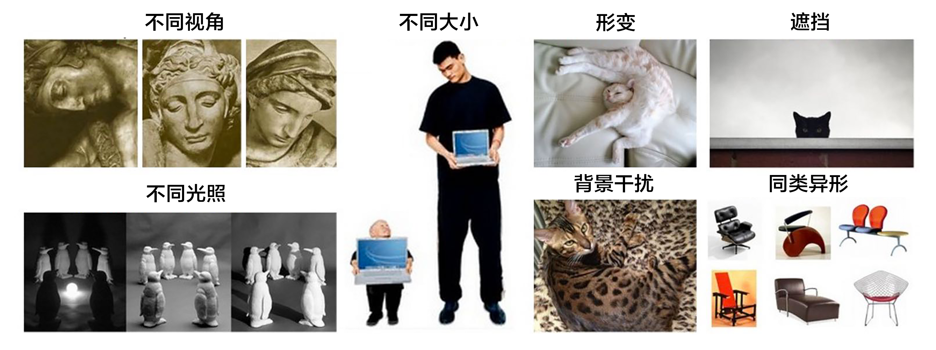
Figure 3. Disturbed images [22]
## Exploration of Models
A large amount of researches in image classification are built upon benchmark datasets such as [PASCAL VOC](http://host.robots.ox.ac.uk/pascal/VOC/), [ImageNet](http://image-net.org/) etc. Many image classification algorithms are usually evaluated and compared based on these datasets. PASCAL VOC is a computer vision competition started in 2005, and ImageNet is a dataset holding Large Scale Visual Recognition Challenge (ILSVRC) started in 2010. In this chapter, we introduce some image classification models from the submissions to these competitions.
Before 2012, traditional image classification was accomplished with the three steps described in the background section. A complete model construction usually involves the following stages: low-level feature extraction, feature encoding, spatial constraint or feature clustering, classifier design, model ensemble.
1). **Low-level feature extraction**: This step extracts large amounts of local features according to fixed strides and scales. Popular local features include Scale-Invariant Feature Transform (SIFT) \[[1](#References)\], Histogram of Oriented Gradient(HOG) \[[2](#References)\], Local Binary Pattern(LBP) \[[3](#References)\], etc. A common practice is to employ multiple feature descriptors in order to avoid missing a lot of information.
2). **Feature encoding**: Low-level features contain a large amount of redundancy and noise. In order to improve the robustness of features, it is necessary to employ a feature transformation to encode low-level features. This is called feature encoding. Common feature encoding methods include vector quantization \[[4](#References)\], sparse coding \[[5](#References)\], locality-constrained linear coding \[[6](#References)\], Fisher vector encoding \[[7](#References)\], etc.
3). **Spatial constraint**: Spatial constraint or feature clustering is usually adopted after feature encoding for extracting the maximum or average of each dimension in the spatial domain. Pyramid feature matching--a popular feature clustering method--divides an image uniformly into patches and performs feature clustering in each patch.
4). **Classification**: In the above steps an image can be described by a vector of fixed dimension. Then a classifier can be used to classify the image into categories. Common classifiers include Support Vector Machine(SVM), random forest etc. Kernel SVM is the most popular classifier and has achieved very good performance in traditional image classification tasks.
This classic method has been used widely as image classification algorithm in PASCAL VOC \[[18](#References)\]. [NEC Labs](http://www.nec-labs.com/) won the championship by employing SIFT and LBP features, two non-linear encoders and SVM in ILSVRC 2010 \[[8](#References)\].
The CNN model--AlexNet proposed by Alex Krizhevsky et al. \[[9](#References)\], made a breakthrough in ILSVRC 2012. It dramatically outperformed classical methods and won the ILSVRC championship in 2012. This was also the first time that a deep learning method was adopted for large-scale image classification. Since AlexNet, a series of CNN models have been proposed that have advanced the state of the art steadily on Imagenet as shown in Figure 4. With deeper and more sophisticated architectures, Top-5 error rate is getting lower and lower (to around 3.5%). The error rate of human raters on the same Imagenet dataset is 5.1%, which means that the image classification capability of a deep learning model has surpassed human raters.
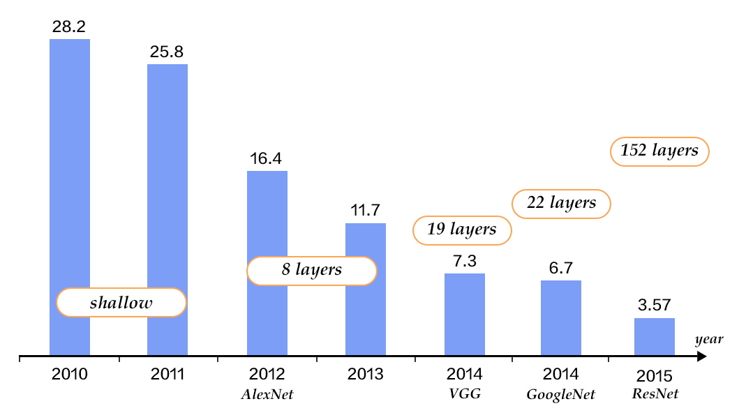
Figure 4. Top-5 error rates on ILSVRC image classification
### CNN
Traditional CNNs consist of convolution and fully-connected layers and use the softmax multi-category classifier with the cross-entropy loss function. Figure 5 shows a typical CNN. We first take look at the common components of a CNN.

Figure 5. A CNN example [20]
- convolutional layer: this layer uses the convolution operation to extract (low-level and high-level) features and to discover local correlation and spatial invariance.
- pooling layer: this layer down-samples feature maps by extracting local max (max-pooling) or average (avg-pooling) value of each patch in the feature map. Down-sampling is a common operation in image processing and is used to filter out trivial high-frequency information.
- fully-connected layer: this layer fully connects neurons between two adjacent layers.
- non-linear activation: Convolutional and fully-connected layers are usually followed by some non-linear activation layers. Non-linearities enhance the expression capability of the network. Some examples of non-linear activation functions are Sigmoid, Tanh and ReLU. ReLU is the most commonly used activation function in CNN.
- Dropout \[[10](#References)\]: At each training stage, individual nodes are dropped out of the network with a certain random probability. This improves the network's ability to generalize and avoids overfitting.
Parameter updates at each layer during training causes input layer distributions to change and in turn requires hyper-parameters to be carefully tuned. In 2015, Sergey Ioffe and Christian Szegedy proposed a Batch Normalization (BN) algorithm \[[14](#References)\], which normalizes the features of each batch in a layer, and enables relatively stable distribution in each layer. Not only does BN algorithm act as a regularizer, but also eliminates the need for meticulous hyper-parameter design. Experiments demonstrate that BN algorithm accelerates the training convergence and has been widely used in further deeper models.
In the following sections, we will take a tour through the following network architectures - VGG, GoogLeNet and ResNets.
### VGG
The Oxford Visual Geometry Group (VGG) proposed the VGG network in ILSVRC 2014 \[[11](#References)\]. This model is deeper and wider than previous neural architectures. Its major part is the five main groups of convolution operations. Adjacent convolution groups are connected via max-pooling layers to perform dimensionality reduction. Each group contains a series of 3x3 convolutional layers (i.e. kernels). The number of convolution kernels stays the same within the single group and increases from 64 in the first group to 512 in the last one. Double FC layers and a classifier layer will follow afterwards. The total number of learnable layers could be 11, 13, 16, or 19 depending on the number of convolutional layers in each group. Figure 6 illustrates a 16-layer VGG. The architecture of VGG is relatively simple and has been adopted by many papers such as the first one that surpassed human-level performance on ImageNet \[[19](#References)\].
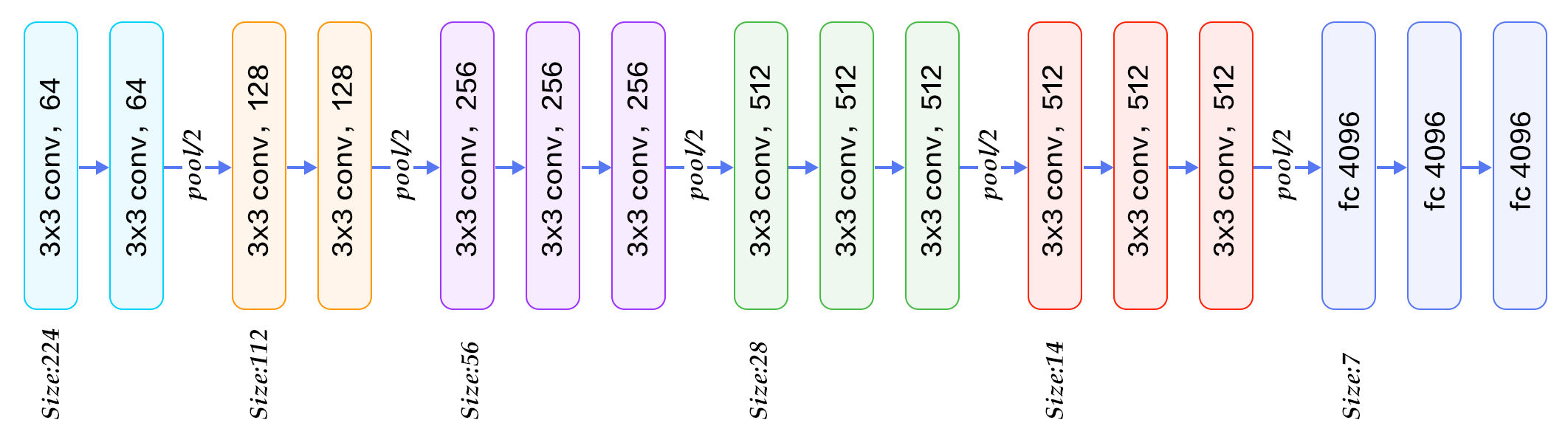
Figure 6. VGG16 model for ImageNet
### GoogLeNet
GoogLeNet \[[12](#References)\] won the ILSVRC championship in 2014. GoogLeNet borrowed some ideas from the Network in Network(NIN) model \[[13](#References)\] and is built on the Inception blocks. Let us first familiarize ourselves with these concepts first.
The two main characteristics of the NIN model are:
1) A single-layer convolutional network is replaced with a Multi-Layer Perceptron Convolution (MLPconv). MLPconv is a tiny multi-layer convolutional network. It enhances non-linearity by adding several 1x1 convolutional layers after linear ones.
2) In traditional CNNs, the last fewer layers are usually fully-connected with a large number of parameters. In contrast, the last convolution layer of NIN contains feature maps of the same size as the category dimension, and NIN replaces fully-connected layers with global average pooling to fetch a vector of the same size as category dimension and classify them. This replacement of fully-connected layers significantly reduces the number of parameters.
Figure 7 depicts two Inception blocks. Figure 7(a) is the simplest design. The output is a concatenation of features from three convolutional layers and one pooling layer. The disadvantage of this design is that the pooling layer does not change the number of channels and leads to an increased channel number of features after concatenation. After several such blocks, the number of channels and parameters become larger and larger and lead to higher computation complexity. To overcome this drawback, the Inception block in Figure 7(b) employs three 1x1 convolutional layers to perform dimensionality reduction, which, to put it simply, is to reduce the number of channels and simultaneously improve the non-linearity of the network.

Figure 7. Inception block
GoogLeNet comprises multiple stacked Inception blocks followed by an avg-pooling layer as in NIN instead of traditional fully connected layers. The difference between GoogLeNet and NIN is that GoogLeNet adds a fully connected layer after avg-pooling layer to output a vector of category size. Besides these two characteristics, the features from middle layers of a GoogLeNet are also very discriminative. Therefore, GoogeleNet inserts two auxiliary classifiers in the model for enhancing gradient and regularization when doing back-propagation. The loss function of the whole network is the weighted sum of these three classifiers.
Figure 8 illustrates the neural architecture of a GoogLeNet which consists of 22 layers: it starts with three regular convolutional layers followed by three groups of sub-networks -- the first group contains two Inception blocks, the second group has five, and the third group has two again. Finally, It ends with an average pooling and a fully-connected layer.
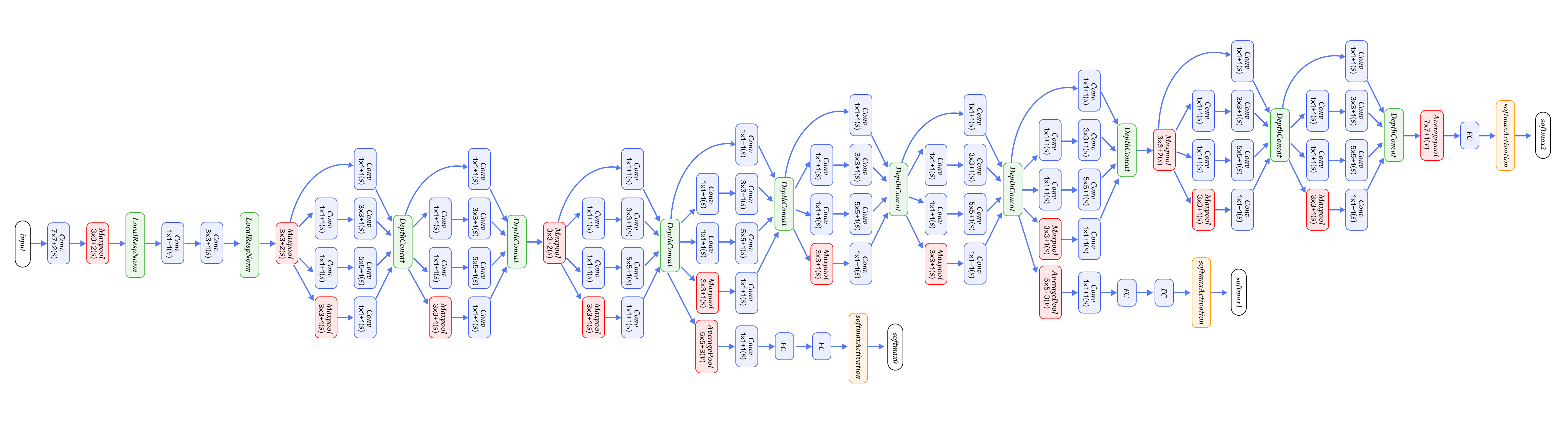
Figure 8. GoogLeNet [12]
The model above is the first version of GoogLeNet or the so-called GoogelNet-v1. GoogLeNet-v2 \[[14](#References)\] introduced BN layer; GoogLeNet-v3 \[[16](#References)\] further split some convolutional layers, which increases non-linearity and network depth; GoogelNet-v4 \[[17](#References)\] is inspired by the design idea of ResNet which will be introduced in the next section. The evolution from v1 to v4 improved the accuracy rate consistently. The length of this article being limited, we will not scrutinize the neural architectures of v2 to v4.
### ResNet
Residual Network(ResNet) \[[15](#References)\] won the 2015 championship on three ImageNet competitions -- image classification, object localization, and object detection. The main challenge in training deeper networks is that accuracy degrades with network depth. The authors of ResNet proposed a residual learning approach to ease the training of deeper networks. Based on the design ideas of BN, small convolutional kernels, full convolutional network, ResNets reformulate the layers as residual blocks, with each block containing two branches, one directly connecting input to the output, the other performing two to three convolutions and calculating the residual function with reference to the layer's inputs. The output features of these two branches are then added up.
Figure 9 illustrates the ResNet architecture. To the left is the basic building block, it consists of two 3x3 convolutional layers with the same size of output channels. To the right is a Bottleneck block. The bottleneck is a 1x1 convolutional layer used to reduce dimension (from 256 to 64 here). The following 1x1 convolutional layer is used to increase dimension from 64 to 256. Thus, the number of input and output channels of the middle 3x3 convolutional layer is relatively small (64->64 in this example).
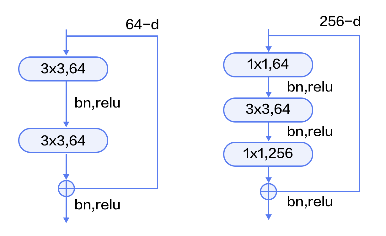
Figure 9. Residual block
Figure 10 illustrates ResNets with 50, 101, 152 layers, respectively. All three networks use bottleneck blocks and their difference lies in the repetition time of residual blocks. ResNet converges very fast and can be trained with hundreds or thousands of layers.

Figure 10. ResNet model for ImageNet
## Get Data Ready
Common public benchmark datasets for image classification are [CIFAR](https://www.cs.toronto.edu/~kriz/cifar.html), [ImageNet](http://image-net.org/), [COCO](http://mscoco.org/), etc. Those used for fine-grained image classification are [CUB-200-2011](http://www.vision.caltech.edu/visipedia/CUB-200-2011.html), [Stanford Dog](http://vision.stanford.edu/aditya86/ImageNetDogs/), [Oxford-flowers](http://www.robots.ox.ac.uk/~vgg/data/flowers/), etc. Among these, the ImageNet dataset is the largest. Most research results are reported on ImageNet as mentioned in the "Exploration of Models" section. Since 2010, the ImageNet dataset has gone through some changes. The commonly used ImageNet-2012 dataset contains 1000 categories. There are 1,281,167 training images, ranging from 732 to 1200 images per category, and 50,000 validation images with 50 images per category in average.
Since ImageNet is too large to be downloaded and trained efficiently, we use [CIFAR-10](https://www.cs.toronto.edu/~kriz/cifar.html) in this tutorial. The CIFAR-10 dataset consists of 60000 32x32 color images in 10 classes, with 6000 images per class. There are 50000 training images and 10000 test images. Figure 11 shows all the classes in CIFAR-10 as well as 10 images randomly sampled from each category.

Figure 11. CIFAR10 dataset [21]
The Paddle API invents 'Paddle.dataset.cifar' to automatically load the Cifar DataSet module.
After running the command `python train.py`, training will start immediately. The following sections will explain `train.py` inside and out.
## Model Configuration
#### Initialize Paddle
Let's start with importing the Paddle Fluid API package and the helper modules.
```python
from __future__ import print_function
import paddle
import paddle.fluid as fluid
import numpy
import sys
```
Now we are going to walk you through the implementations of the VGG and ResNet.
### VGG
Let's start with the VGG model. Since the image size and amount of CIFAR10 are smaller than ImageNet, we tailor our model to fit CIFAR10 dataset. Convolution groups incorporate BN and dropout operations.
The input to VGG core module is the data layer. `vgg_bn_drop` defines a 16-layer VGG network, with each convolutional layer followed by BN and dropout layers. Here is the definition in detail:
```python
def vgg_bn_drop(input):
def conv_block(ipt, num_filter, groups, dropouts):
return fluid.nets.img_conv_group(
input=ipt,
pool_size=2,
pool_stride=2,
conv_num_filter=[num_filter] * groups,
conv_filter_size=3,
conv_act='relu',
conv_with_batchnorm=True,
conv_batchnorm_drop_rate=dropouts,
pool_type='max')
conv1 = conv_block(input, 64, 2, [0.3, 0])
conv2 = conv_block(conv1, 128, 2, [0.4, 0])
conv3 = conv_block(conv2, 256, 3, [0.4, 0.4, 0])
conv4 = conv_block(conv3, 512, 3, [0.4, 0.4, 0])
conv5 = conv_block(conv4, 512, 3, [0.4, 0.4, 0])
drop = fluid.layers.dropout(x=conv5, dropout_prob=0.5)
fc1 = fluid.layers.fc(input=drop, size=512, act=None)
bn = fluid.layers.batch_norm(input=fc1, act='relu')
drop2 = fluid.layers.dropout(x=bn, dropout_prob=0.5)
fc2 = fluid.layers.fc(input=drop2, size=512, act=None)
predict = fluid.layers.fc(input=fc2, size=10, act='softmax')
return predict
```
1. Firstly, it defines a convolution block or conv_block. The default convolution kernel is 3x3, and the default pooling size is 2x2 with stride 2. Groups decide the number of consecutive convolution operations in each VGG block. Dropout specifies the probability to perform dropout operation. Function `img_conv_group` is predefined in `paddle.nets` consisting of a series of `Conv->BN->ReLu->Dropout` and a group of `Pooling` .
2. Five groups of convolutions. The first two groups perform two consecutive convolutions, while the last three groups perform three convolutions in sequence. The dropout rate of the last convolution in each group is set to 0, which means there is no dropout for this layer.
3. The last two layers are fully-connected layers of 512 dimensions.
4. The VGG network begins with extracting high-level features and then maps them to a vector of the same size as the category dimension. Finally, Softmax function is used for calculating the probability of classifying the image to each category.
### ResNet
The 1st, 3rd, and 4th step is identical to the counterparts in VGG, which are skipped hereby.
We will explain the 2nd step at lengths, namely the core module of ResNet on CIFAR10.
To start with, here are some basic functions used in `resnet_cifar10` ,and the network connection procedure is illustrated afterwards:
- `conv_bn_layer` : convolutional layer with BN.
- `shortcut` : the shortcut connection in a residual block. There are two kinds of shortcuts: 1x1 convolutions are used to increase dimensionality when in the residual block the number of channels in input feature and that in output feature are different; direct connection used otherwise.
- `basicblock` : a basic residual module as shown in the left of Figure 9, it consists of two sequential 3x3 convolutions and one "shortcut" branch.
- `layer_warp` : a group of residual modules consisting of several stacked blocks. In each group, the sliding window size of the first residual block could be different from the rest, in order to reduce the size of feature maps along horizontal and vertical directions.
```python
def conv_bn_layer(input,
ch_out,
filter_size,
stride,
padding,
act='relu',
bias_attr=False):
tmp = fluid.layers.conv2d(
input=input,
filter_size=filter_size,
num_filters=ch_out,
stride=stride,
padding=padding,
act=None,
bias_attr=bias_attr)
return fluid.layers.batch_norm(input=tmp, act=act)
def shortcut(input, ch_in, ch_out, stride):
if ch_in != ch_out:
return conv_bn_layer(input, ch_out, 1, stride, 0, None)
else:
return input
def basicblock(input, ch_in, ch_out, stride):
tmp = conv_bn_layer(input, ch_out, 3, stride, 1)
tmp = conv_bn_layer(tmp, ch_out, 3, 1, 1, act=None, bias_attr=True)
short = shortcut(input, ch_in, ch_out, stride)
return fluid.layers.elementwise_add(x=tmp, y=short, act='relu')
def layer_warp(block_func, input, ch_in, ch_out, count, stride):
tmp = block_func(input, ch_in, ch_out, stride)
for i in range(1, count):
tmp = block_func(tmp, ch_out, ch_out, 1)
return tmp
```
The following are the components of `resnet_cifar10`:
1. The lowest level is `conv_bn_layer` , e.t. the convolution layer with BN.
2. The next level is composed of three residual blocks, namely three `layer_warp`, each of which uses the left residual block in Figure 10.
3. The last level is average pooling layer.
Note: Except the first convolutional layer and the last fully-connected layer, the total number of layers with parameters in three `layer_warp` should be dividable by 6. In other words, the depth of `resnet_cifar10` should satisfy (depth-2)%6=0.
```python
def resnet_cifar10(ipt, depth=32):
# depth should be one of 20, 32, 44, 56, 110, 1202
assert (depth - 2) % 6 == 0
n = (depth - 2) // 6
nStages = {16, 64, 128}
conv1 = conv_bn_layer(ipt, ch_out=16, filter_size=3, stride=1, padding=1)
res1 = layer_warp(basicblock, conv1, 16, 16, n, 1)
res2 = layer_warp(basicblock, res1, 16, 32, n, 2)
res3 = layer_warp(basicblock, res2, 32, 64, n, 2)
pool = fluid.layers.pool2d(
input=res3, pool_size=8, pool_type='avg', pool_stride=1)
predict = fluid.layers.fc(input=pool, size=10, act='softmax')
return predict
```
## Inference Program Configuration
The input to the network is defined as `fluid.layers.data` , corresponding to image pixels in the context of image classification. The images in CIFAR10 are 32x32 coloured images with three channels. Therefore, the size of the input data is 3072 (3x32x32).
```python
def inference_program():
# The image is 32 * 32 with RGB representation.
data_shape = [3, 32, 32]
images = fluid.layers.data(name='pixel', shape=data_shape, dtype='float32')
predict = resnet_cifar10(images, 32)
# predict = vgg_bn_drop(images) # un-comment to use vgg net
return predict
```
## Training Program Configuration
Then we need to set up the the `train_program`. It takes the prediction from the inference_program first.
During the training, it will calculate the `avg_loss` from the prediction.
In the context of supervised learning, labels of training images are defined in `fluid.layers.data` as well. During training, the multi-class cross-entropy is used as the loss function and becomes the output of the network. During testing, the outputs are the probabilities calculated in the classifier.
**NOTE:** A training program should return an array and the first returned argument has to be `avg_cost` .
The trainer always uses it to calculate the gradients.
```python
def train_program():
predict = inference_program()
label = fluid.layers.data(name='label', shape=[1], dtype='int64')
cost = fluid.layers.cross_entropy(input=predict, label=label)
avg_cost = fluid.layers.mean(cost)
accuracy = fluid.layers.accuracy(input=predict, label=label)
return [avg_cost, accuracy, predict]
```
## Optimizer Function Configuration
In the following `Adam` optimizer, `learning_rate` specifies the learning rate in the optimization procedure. It influences the convergence speed.
```python
def optimizer_program():
return fluid.optimizer.Adam(learning_rate=0.001)
```
## Model Training
### Data Feeders Configuration
`cifar.train10()` generates one sample at a time as the input for training after completing shuffle and batch.
```python
# Each batch will yield 128 images
BATCH_SIZE = 128
# Reader for training
train_reader = paddle.batch(
paddle.reader.shuffle(paddle.dataset.cifar.train10(), buf_size=50000),
batch_size=BATCH_SIZE)
# Reader for testing. A separated data set for testing.
test_reader = paddle.batch(
paddle.dataset.cifar.test10(), batch_size=BATCH_SIZE)
```
### Implementation of the trainer program
We need to develop a main_program for the training process. Similarly, we need to configure a test_program for the test program. It's also necessary to define the `place` of the training and use the optimizer `optimizer_program` previously defined .
```python
use_cuda = False
place = fluid.CUDAPlace(0) if use_cuda else fluid.CPUPlace()
feed_order = ['pixel', 'label']
main_program = fluid.default_main_program()
star_program = fluid.default_startup_program()
avg_cost, acc, predict = train_program()
# Test program
test_program = main_program.clone(for_test=True)
optimizer = optimizer_program()
optimizer.minimize(avg_cost)
exe = fluid.Executor(place)
EPOCH_NUM = 2
# For training test cost
def train_test(program, reader):
count = 0
feed_var_list = [
program.global_block().var(var_name) for var_name in feed_order
]
feeder_test = fluid.DataFeeder(
feed_list=feed_var_list, place=place)
test_exe = fluid.Executor(place)
accumulated = len([avg_cost, acc]) * [0]
for tid, test_data in enumerate(reader()):
avg_cost_np = test_exe.run(program=program,
feed=feeder_test.feed(test_data),
fetch_list=[avg_cost, acc])
accumulated = [x[0] + x[1][0] for x in zip(accumulated, avg_cost_np)]
count += 1
return [x / count for x in accumulated]
```
### The main loop of training and the outputs along the process
In the next main training cycle, we will observe the training process or run test in good use of the outputs.
You can also use `plot` to plot the process by calling back data:
```python
params_dirname = "image_classification_resnet.inference.model"
from paddle.utils.plot import Ploter
train_prompt = "Train cost"
test_prompt = "Test cost"
plot_cost = Ploter(test_prompt,train_prompt)
# main train loop.
def train_loop():
feed_var_list_loop = [
main_program.global_block().var(var_name) for var_name in feed_order
]
feeder = fluid.DataFeeder(
feed_list=feed_var_list_loop, place=place)
exe.run(star_program)
step = 0
for pass_id in range(EPOCH_NUM):
for step_id, data_train in enumerate(train_reader()):
avg_loss_value = exe.run(main_program,
feed=feeder.feed(data_train),
fetch_list=[avg_cost, acc])
if step % 1 == 0:
plot_cost.append(train_prompt, step, avg_loss_value[0])
plot_cost.plot()
step += 1
avg_cost_test, accuracy_test = train_test(test_program,
reader=test_reader)
plot_cost.append(test_prompt, step, avg_cost_test)
# save parameters
if params_dirname is not None:
fluid.io.save_inference_model(params_dirname, ["pixel"],
[predict], exe)
```
### Training
Training via `trainer_loop` function, here we only have 2 Epoch iterations. Generally we need to execute above a hundred Epoch in practice.
**Note:** On CPU, each Epoch will take approximately 15 to 20 minutes. It may cost some time in this part. Please freely update the code and run test on GPU to accelerate training
```python
train_loop()
```
An example of an epoch of training log is shown below. After 1 pass, the average Accuracy on the training set is 0.59 and the average Accuracy on the testing set is 0.6.
```text
Pass 0, Batch 0, Cost 3.869598, Acc 0.164062
...................................................................................................
Pass 100, Batch 0, Cost 1.481038, Acc 0.460938
...................................................................................................
Pass 200, Batch 0, Cost 1.340323, Acc 0.523438
...................................................................................................
Pass 300, Batch 0, Cost 1.223424, Acc 0.593750
..........................................................................................
Test with Pass 0, Loss 1.1, Acc 0.6
```
Figure 13 is a curve graph of the classification error rate of the training. After pass of 200 times, it almost converges, and finally the classification error rate on the test set is 8.54%.
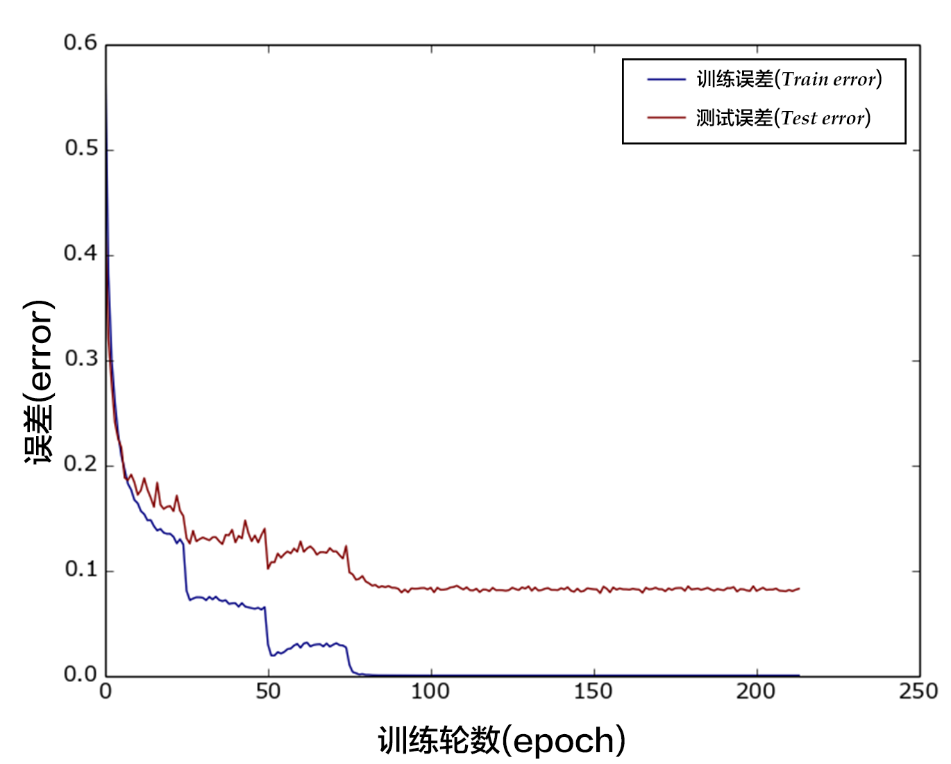
Figure 13. Classification error rate of VGG model on the CIFAR10 data set
## Model Application
You can use a trained model to classify your images. The following program shows how to load a trained network and optimized parameters for inference.
### Generate Input Data to infer
`dog.png` is a picture of a puppy. We convert it to a `numpy` array to meet the `feeder` format.
```python
# Prepare testing data.
from PIL import Image
import os
def load_image(file):
im = Image.open(file)
im = im.resize((32, 32), Image.ANTIALIAS)
im = numpy.array(im).astype(numpy.float32)
# The storage order of the loaded image is W(width),
# H(height), C(channel). PaddlePaddle requires
# the CHW order, so transpose them.
im = im.transpose((2, 0, 1)) # CHW
im = im / 255.0
# Add one dimension to mimic the list format.
im = numpy.expand_dims(im, axis=0)
return im
cur_dir = os.getcwd()
img = load_image(cur_dir + '/image/dog.png')
```
### Inferencer Configuration and Inference
Similar to the training process, a inferencer needs to build the corresponding process. We load the trained network and parameters from `params_dirname` .
We can just insert the inference program defined previously.
Now let's make our inference.
```python
place = fluid.CUDAPlace(0) if use_cuda else fluid.CPUPlace()
exe = fluid.Executor(place)
inference_scope = fluid.core.Scope()
with fluid.scope_guard(inference_scope):
[inference_program, feed_target_names,
fetch_targets] = fluid.io.load_inference_model(params_dirname, exe)
# Construct feed as a dictionary of {feed_target_name: feed_target_data}
# and results will contain a list of data corresponding to fetch_targets.
results = exe.run(inference_program,
feed={feed_target_names[0]: img},
fetch_list=fetch_targets)
# infer label
label_list = [
"airplane", "automobile", "bird", "cat", "deer", "dog", "frog", "horse",
"ship", "truck"
]
print("infer results: %s" % label_list[numpy.argmax(results[0])])
```
## Summary
The traditional image classification method consists of multiple stages. The framework is a little complex. In contrast, the end-to-end CNN model can be implemented in one step, and the accuracy of classification is greatly improved. In this article, we first introduced three classic models, VGG, GoogLeNet and ResNet. Then we have introduced how to use PaddlePaddle to configure and train CNN models based on CIFAR10 dataset, especially VGG and ResNet models. Finally, we have guided you how to use PaddlePaddle's API interfaces to predict images and extract features. For other datasets such as ImageNet, the configuration and training process is the same, so you can embark on your adventure on your own.
## References
[1] D. G. Lowe, [Distinctive image features from scale-invariant keypoints](http://www.cs.ubc.ca/~lowe/papers/ijcv04.pdf). IJCV, 60(2):91-110, 2004.
[2] N. Dalal, B. Triggs, [Histograms of Oriented Gradients for Human Detection](http://vision.stanford.edu/teaching/cs231b_spring1213/papers/CVPR05_DalalTriggs.pdf), Proc. IEEE Conf. Computer Vision and Pattern Recognition, 2005.
[3] Ahonen, T., Hadid, A., and Pietikinen, M. (2006). [Face description with local binary patterns: Application to face recognition](http://ieeexplore.ieee.org/document/1717463/). PAMI, 28.
[4] J. Sivic, A. Zisserman, [Video Google: A Text Retrieval Approach to Object Matching in Videos](http://www.robots.ox.ac.uk/~vgg/publications/papers/sivic03.pdf), Proc. Ninth Int'l Conf. Computer Vision, pp. 1470-1478, 2003.
[5] B. Olshausen, D. Field, [Sparse Coding with an Overcomplete Basis Set: A Strategy Employed by V1?](http://redwood.psych.cornell.edu/papers/olshausen_field_1997.pdf), Vision Research, vol. 37, pp. 3311-3325, 1997.
[6] Wang, J., Yang, J., Yu, K., Lv, F., Huang, T., and Gong, Y. (2010). [Locality-constrained Linear Coding for image classification](http://ieeexplore.ieee.org/abstract/document/5540018/). In CVPR.
[7] Perronnin, F., Sánchez, J., & Mensink, T. (2010). [Improving the fisher kernel for large-scale image classification](http://dl.acm.org/citation.cfm?id=1888101). In ECCV (4).
[8] Lin, Y., Lv, F., Cao, L., Zhu, S., Yang, M., Cour, T., Yu, K., and Huang, T. (2011). [Large-scale image clas- sification: Fast feature extraction and SVM training](http://ieeexplore.ieee.org/document/5995477/). In CVPR.
[9] Krizhevsky, A., Sutskever, I., and Hinton, G. (2012). [ImageNet classification with deep convolutional neu- ral networks](http://www.cs.toronto.edu/~kriz/imagenet_classification_with_deep_convolutional.pdf). In NIPS.
[10] G.E. Hinton, N. Srivastava, A. Krizhevsky, I. Sutskever, and R.R. Salakhutdinov. [Improving neural networks by preventing co-adaptation of feature detectors](https://arxiv.org/abs/1207.0580). arXiv preprint arXiv:1207.0580, 2012.
[11] K. Chatfield, K. Simonyan, A. Vedaldi, A. Zisserman. [Return of the Devil in the Details: Delving Deep into Convolutional Nets](https://arxiv.org/abs/1405.3531). BMVC, 2014。
[12] Szegedy, C., Liu, W., Jia, Y., Sermanet, P., Reed, S., Anguelov, D., Erhan, D., Vanhoucke, V., Rabinovich, A., [Going deeper with convolutions](https://arxiv.org/abs/1409.4842). In: CVPR. (2015)
[13] Lin, M., Chen, Q., and Yan, S. [Network in network](https://arxiv.org/abs/1312.4400). In Proc. ICLR, 2014.
[14] S. Ioffe and C. Szegedy. [Batch normalization: Accelerating deep network training by reducing internal covariate shift](https://arxiv.org/abs/1502.03167). In ICML, 2015.
[15] K. He, X. Zhang, S. Ren, J. Sun. [Deep Residual Learning for Image Recognition](https://arxiv.org/abs/1512.03385). CVPR 2016.
[16] Szegedy, C., Vanhoucke, V., Ioffe, S., Shlens, J., Wojna, Z. [Rethinking the incep-tion architecture for computer vision](https://arxiv.org/abs/1512.00567). In: CVPR. (2016).
[17] Szegedy, C., Ioffe, S., Vanhoucke, V. [Inception-v4, inception-resnet and the impact of residual connections on learning](https://arxiv.org/abs/1602.07261). arXiv:1602.07261 (2016).
[18] Everingham, M., Eslami, S. M. A., Van Gool, L., Williams, C. K. I., Winn, J. and Zisserman, A. [The Pascal Visual Object Classes Challenge: A Retrospective](http://link.springer.com/article/10.1007/s11263-014-0733-5). International Journal of Computer Vision, 111(1), 98-136, 2015.
[19] He, K., Zhang, X., Ren, S., and Sun, J. [Delving Deep into Rectifiers: Surpassing Human-Level Performance on ImageNet Classification](https://arxiv.org/abs/1502.01852). ArXiv e-prints, February 2015.
[20] http://deeplearning.net/tutorial/lenet.html
[21] https://www.cs.toronto.edu/~kriz/cifar.html
[22] http://cs231n.github.io/classification/

This tutorial is contributed by PaddlePaddle, and licensed under a Creative Commons Attribution-ShareAlike 4.0 International License.